Start to end prototype example

This example shows a start to end workflow which begins with detecting calls across channels in an audio file, and then moving to localising the call positions. It ends with a display of the localised positions in comparison with the original simulated positions.

import batracker
from batracker.localisation import friedlander_1987 as fr87
import matplotlib.pyplot as plt
plt.rcParams['agg.path.chunksize']=10000
from mpl_toolkits.mplot3d import Axes3D
import numpy as np
import pandas as pd
import scipy.io.wavfile as wavfile
from batracker.signal_detection import detection
from batracker.correspondence_matching import multichannel_match as matching
from batracker.tdoa_estimation import tdoa_estimators

Load the simulated audio file

import tacost
from tacost import calculate_toa as ctoa

Generate an array geometry and use simulated source positions

mic_positions = np.array([[ 0, 0, 0],
                          [ 1, 0, 0],
                          [-1, 1, 0],
                          [ 0, 0.5, 0],
                          [-2,2,1]
                       ])

x = np.linspace(2,10,3)
y = x.copy()
z = x.copy()

xyz = np.array(np.meshgrid(x,y,z)).T.reshape(-1,3)

test_pos = xyz
toa = ctoa.calculate_mic_arrival_times(test_pos,
                                       array_geometry=mic_positions,
                                       intersound_interval=0.05)

test_audio, fs = tacost.make_sim_audio.create_audio_for_mic_arrival_times(toa,
                                                        call_snr=80)
audio = test_audio.copy()

Detect the calls in each channel

detections = detection.cross_channel_threshold_detector(audio, fs,
                                              dbrms_window=0.5*10**-3,
                                              dbrms_threshold=-60)

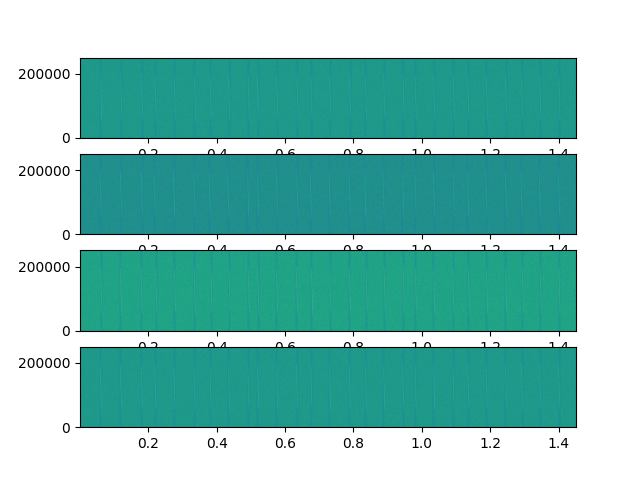
# Spectrogram of the cross-corr boundaries
plt.figure()
ax= plt.subplot(411)
plt.specgram(audio[:,0], Fs=fs)
for each in detections[0]:
    plt.vlines(each, 0, fs*0.5, linewidth=0.2)

for i in range(2,5):
    plt.subplot(410+i, sharex=ax)
    plt.specgram(audio[:,i-1], Fs=fs)
    for each in detections[i-1]:
        plt.vlines(each, 0, fs*0.5, linewidth=0.2)


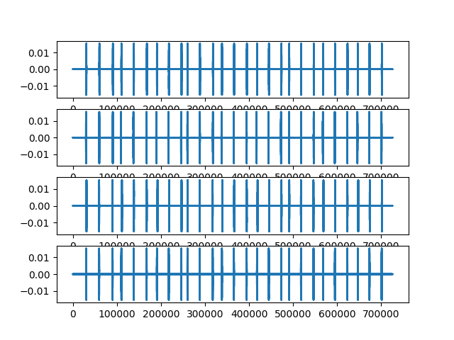
# Waveformsof the detection

plt.figure()
ax= plt.subplot(411)
plt.plot(audio[:,0])
for each in detections[0]:
    plt.vlines(np.array(each)*fs, np.min(audio), np.max(audio), 'k',linewidth=0.5)

for i in range(2,5):
    plt.subplot(410+i, sharex=ax)
    plt.plot(audio[:,i-1])
    for each in detections[i-1]:
        plt.vlines(np.array(each)*fs,
                   np.min(audio), np.max(audio), 'k',linewidth=0.5)

• 
• 

Out:

5 725707

  0%|          | 0/5 [00:00<?, ?it/s]
 20%|##        | 1/5 [00:11<00:47, 11.90s/it]
 40%|####      | 2/5 [00:23<00:35, 11.95s/it]
 60%|######    | 3/5 [00:35<00:23, 11.96s/it]
 80%|########  | 4/5 [00:47<00:11, 11.90s/it]
100%|##########| 5/5 [00:59<00:00, 11.92s/it]
100%|##########| 5/5 [00:59<00:00, 11.92s/it]

The cross-cor boundary needs to be calculated keeping the whole signal duration in mind too!!

Perform correspondence matching and generate the common boundaries across channels for cross=correlation. Also, load the mic array geometry as the max- inter-mic distances are required for the calculation of max inter-mic delays

ag = pd.DataFrame(mic_positions)
ag.columns  = ['x','y','z']

crosscor_boundaries = matching.generate_crosscor_boundaries(detections, ag)

num_channels = audio.shape[1]

Estimate time-difference-of-arrival across different channels and sounds

reference_ch = 3

all_tdoas = {}
for i,each_common in enumerate(crosscor_boundaries):
    start, stop = each_common
    start_sample, stop_sample = int(start*fs), int(stop*fs)

    tdoas = tdoa_estimators.measure_tdoa(audio[start_sample:stop_sample,:], fs, ref_channel=reference_ch)
    all_tdoas[i] = tdoas

Use the TDOAs to calculate positions of sound sources

vsound = 338.0
all_positions = []
num_rows = mic_positions.shape[0]-1
calculated_positions = np.zeros((test_pos.shape[0], 3))
for det_number, tdoas in all_tdoas.items():
    try:
        d = vsound*tdoas
        pos = fr87.solve_friedlander1987(mic_positions, d, j=reference_ch,
                                         use_analytical=False).flatten()
        calculated_positions[det_number,:] = pos
    except:
        print(f'COULD NOT CALCULATE POSITION FOR TEST POSITION {det_number}')

Out:

/home/docs/checkouts/readthedocs.org/user_builds/batracker/checkouts/latest/batracker/localisation/friedlander_1987.py:100: FutureWarning: `rcond` parameter will change to the default of machine precision times ``max(M, N)`` where M and N are the input matrix dimensions.
To use the future default and silence this warning we advise to pass `rcond=None`, to keep using the old, explicitly pass `rcond=-1`.
  xs,resid, _,_ = np.linalg.lstsq(MjSj, Mjmuj)

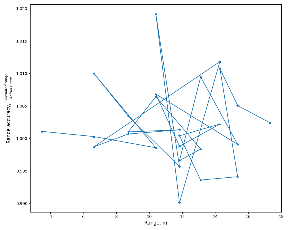
Accuracy

Now let’s estimate the accuracy of the positions in general, in terms of their ranges from the origin.

test_ranges = np.apply_along_axis(fr87.distance_to_point, 1, test_pos, [0,0,0])
calc_ranges = np.apply_along_axis(fr87.distance_to_point, 1, calculated_positions, [0,0,0])

range_accuracy = calc_ranges/test_ranges

plt.figure(figsize=(10,8))
plt.plot(test_ranges, range_accuracy, '-*')
plt.ylabel('Range accuracy, $\\frac{Calculated\ range}{Actual\ range}$', fontsize=12)
plt.xlabel('Range, m', fontsize=12)
plt.tight_layout()

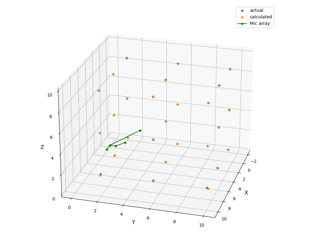
fig = plt.figure(figsize=(10,8))
ax = fig.add_subplot(111, projection='3d')
ax.view_init(elev=24, azim=16)
ax.plot(test_pos[:,0], test_pos[:,1], test_pos[:,2],'*', label='actual')
ax.plot(calculated_positions[:,0], calculated_positions[:,1],
        calculated_positions[:,2],'*', label='calculated')

ax.plot(mic_positions[0:2,0], mic_positions[0:2,1],
        mic_positions[0:2,2],'g-*')
ax.plot(mic_positions[2:4,0], mic_positions[2:4,1],
        mic_positions[2:4,2],'g-*')
ax.plot(mic_positions[[0,4],0], mic_positions[[0,4],1],
        mic_positions[[0,4],2],'g-*')
ax.plot(mic_positions[[0,3],0], mic_positions[[0,3],1],
        mic_positions[[0,3],2],'g-*', label='Mic array')
plt.legend()
plt.tight_layout()
ax.set_xlabel('X', fontsize=12);ax.set_ylabel('Y', fontsize=12); ax.set_zlabel('Z', fontsize=12)

• 
• 

Out:

Text(0.5, 0, 'Z')